Notes on speech from signal processing perspective
DRAFT: This post is a work in progress. Not finished yet.
The ideal multimodal agent would integrate an audio processing system. I decided to share some notes on speech,starting from a signal procesing perspective.
NOTE: This is a very high-level overview. Will use minial math notation.
- Talk about how to sample a wave form, period, sampling frequency, and FFTs etc.
Ah, yes. Information! Don’t we all love information? from the tiniest level of organization (neucleotide sequence in DNA) to the high bitrate transfer of bitstreams between different memory compartments in a classical Von Neumman architected computer. Information is akin to manna, analogized over a metallo-silicon substrate. Today though, i’d like to dive into a specific form of information, sound. Sound is a pretty weird one because it’s not at all a tangible physical quantity, but it is very much ubiquitious in our physical system. Starting from the definitation of waves, and fields, we can define “sound” as a the phenomenon produced by pertubations of the air, ie vibrations propagated through the air, like any other wave over it’s medium.
To approach this from a more information theoretic persperctive, we call upon the inital information propagation pipeline as denoted by Shannon:
- Let the source S, be the set containing the list of states that one can conceive as letters of a primitive alphabet.
- Let the encoder E, be the encoding function that transforms the written or spoken message into bits of information to be transmitted.
- Let the channel CH, be the medium by which said encoded signal passes.
- Let receiver R, be the decoding function that decompresses the encoded signal to be received by the destination.
- Let the destination D, be the entity receiving said message.
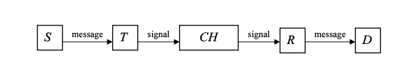
Figure 1. A Canonical information propagation system as denoted by Shannon & Weaver in “The mathematical theory of communication”
To return to more applicable means. In the field of signal processing, primarily, digital signal processing, a common and somewhat indispensable method is that of signal transformation between different domains (ie, frequency, time, amplitude, etc). Generally speaking, input signals of any form are usually exist in a continious form, meaning that in order to use such an input signal at any capacity, we would have to initally convert it into a dicsrete repesenatation. This is where sampling a continous signal somes into play!
We all know what sampling is. Sweet sweet sampling. I’m sorry, I just really love any sort of sparsification or compression type derivative. In this case, given the set of all points in the continous input signal, we discriminately select samples of the set by a sampling criterion denoted by 1/Fs (period), where Fs is the sampling frequency. More formally:
let the raw input signal be defined as X(t), where t is the time variable. Using the sampling criterion, we collect n samples from X(t) at a rate of Fs per second. The output of this gives us our number of sampled points (which, again is quite heavily dependent on the sampling frequency used. Will talk more about this as we proceed). Then we proceed to normalize our samped points in time with Ts = 1/Fs to obtain the discretized version X[n], were n is the number of samples, of the inital continous raw input. Finally, with this discretized version of the inital input, we can work our digital magic on it!
Illustration:
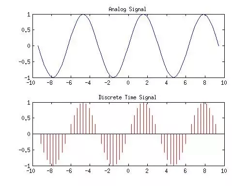
Fig 2. The process illustrated above is conducted by any general analog-ti-digital conversion system. Just sample points with a sample rate criterion, measured in KHz, then we get the discretized version that we can actually run computations on.
Note: For the purpose of running computations on human audio, we generally, as a rule of thumb, use a sampling rate of aobut 16000KHz.
Ok, now we can get inrto the meat of things. We’ve now seen how to convert a raw continous input signal into a discretized version for better computation over a digital substrate, now we look at the algorithms that actually allow us to process X[n]. In the space of dicrete signal processing - or more specifically, Fourier analysis on discrete-time signals, we have these fourier transforms called DFT (Discrete Fourier Transform), and DTFT (Discrete Time Fourier Transform).
Canonically, the DTFT of a raw input signal undergoes two intermediary transformation before DFT being computed.
We denote the DTFT of an input sequence, X[n] to be:

where  denotes the raw input signal as a continous function of omega. So as we saw above, we have to sample points on based on the sampling criteria we defined above, 1/Fs. Recall that we do such a sampling to discretize the inital raw input signal. Note that sampling of raw signal occurs in frequency domain.
Upon application of DTFT algorithm, we
denotes the raw input signal as a continous function of omega. So as we saw above, we have to sample points on based on the sampling criteria we defined above, 1/Fs. Recall that we do such a sampling to discretize the inital raw input signal. Note that sampling of raw signal occurs in frequency domain.
Upon application of DTFT algorithm, we
-
Move on to short time fourier transforms, and how that works, and why to use it in place of canonical FFTs.
-
Move on to mel spectrograms, and how they can be decoded.
-
Do a thorough account of Vocoders (nerual vocoders). Talk about different backbones and their advantages and drawbacks
References
- DSPGAN: a GAN-based universal vocoder for high-fidelity TTS by time-frequency domain supervision from DSP
- SpecGrad: Diffusion Probabilistic Model based Neural Vocoder with Adaptive Noise Spectral Shaping
- TorToiSe Architectural Design Doc
- CMU - Notes on Short-Time Fourier Transforms
- Wikipedia - Discrete Fourier Transform
- Wikipedia = Fast Fourier Transform